
One of our research interests is the sonic logging technique: the employment of acoustic waves in fluid-filled boreholes for Geophysics and Petrophysics applications. Together with our collaborators, we simulate the propagation of acoustic modes in boreholes using finite element method (FEM) as well as implement numerical algorithms for field data post-processing. In this way, we use computational methods to treat field acquired data and physical simulations for data interpretation.
Research overview
In sonic logging, one uses boreholes with approximately 10 cm radii and few kilometers depth to probe the surrounding geological formation. The idea is use a cylindrical looging tool to launch and detect acoustic bursts which propagate through system carrying information about the surrounding medium. From the time dependent collected signals, we are able to estimate the elastic properties the formation like propagation velocities, porosity, and permeability. More sophisticated acquisition procedures also provide information about anisotropies, fractures, and the presence of hydrocarbons [1].
One of our interests is to use numerical methods to simulate real data acquisition. This is not an easy task due to the large number of factors and uncertainties involved in this kind of experiment. Therefore, we start with simplified models and add complexity to them according to the case of interest.
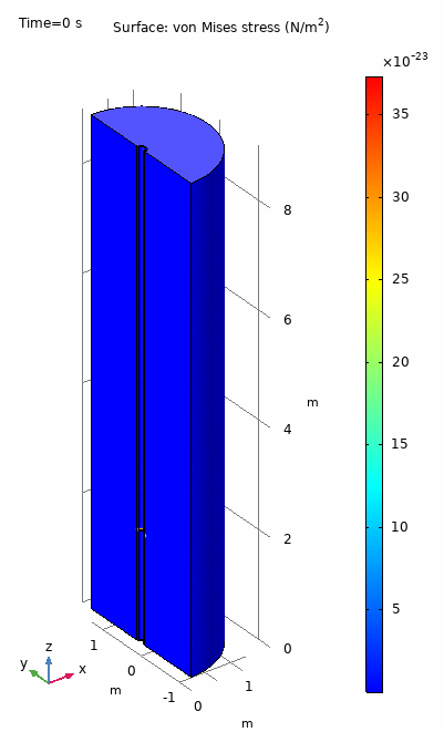
The animation below is a FEM simulation of a real logging tool experiment. A short wave pulse generated by a monopole source propagates through the fluid and surrounding formation. We can observe different modes with distinct propagation velocities inducing different deformation fields in the system. The information is collected an array of equally spaced detectors which generate and time dependent signal. In experiments, this signal is processed and the dispersion curves of the main propagating modes are obtained.
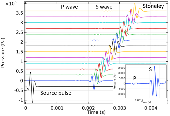
The simulated time dependent signal detected the array, the so called waveform chart, is shown below. The black curve is the pulse generated by the source and the colored curves are the time response of each one of the 13 detectors which form the array. We can clear observe the arrivals of three wavefronts corresponding to the compressional (P), shear (S), and guided (Stoneley) modes.
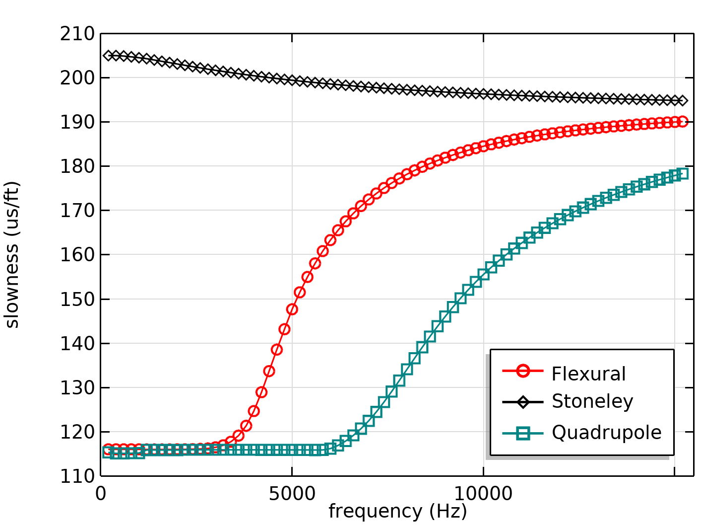
We also employ modal analysis to check the presence of higher order modes in the system. The figure below shows the calculated dispersion curves of the three main guided modes in the formation: Stoneley, flexural, and quadrupole modes. The slowness is the inverse of the velocity of the wave. Each dispersion curve carries different information about each mode. The flexural mode is of high interest in Geophysics due its use in the calculation of the shear wave slowness in the low frequency regime.
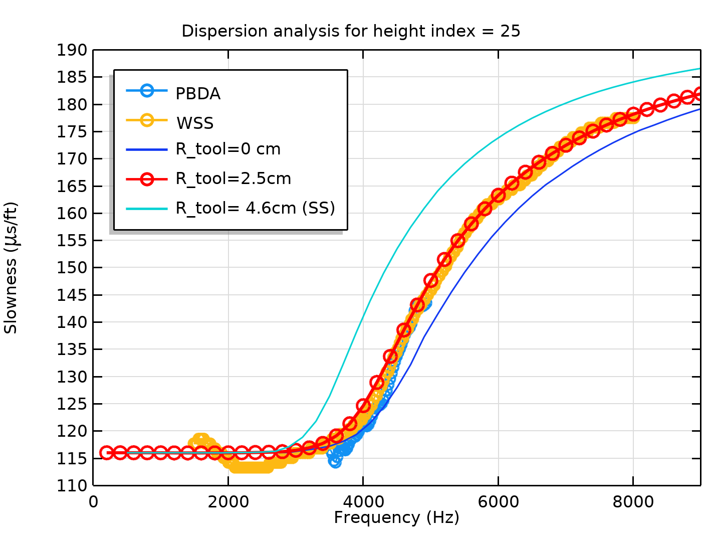
The figure shown in the sequence is an application of FEM simulation for real data analysis of the flexural mode dispersion curve. This an example of application of the equivalent tool theory method. The blue (PBDA) and orange (WSS) points are post-processed experimental data. The other three curves are FEM simulations. The blue curve is the dispersion relation which would be expected if the borehole was only filled with the fluid. The cyan dispersion take into account the presence of a real tool with its nominal radius of 4.6 cm inside the borehole. The red circle dispersion is an adjustment of the experimental data with an effective tool radius of 2.5 cm. This is a very employed method and it is justified because the tool is not an homogeneous solid object and, in most of the cases, is also filled with fluid. As we observe, the simulation is able to reproduce the acquired data reasonably and allows us to estimate the shear wave velocity of the formation in the low frequency limit.
[1] J. B. U. Haldorsen, et. al, Borehole Acoustic Waves, Oilfield Review (2006)


Comentários